Stableswaps from the desk of Alexander Szul

Following my conversation with Jomari, the Core Strategist of Axial and Snowball, I was asked by my team for a deeper dive into the technical details of “stableswaps”. Happy to oblige, I will be going into further detail about the purposes behind stableswaps and stable assets and how they function. To watch the full discussion with Jomari, click here.

Stable Assets

In an ecosystem as volatile as DeFi, it is important that traders of all sizes can enter into a sense of stability without needing to cash out their crypto. Not only does transferring crypto to cash take time, but it also can become rather expensive due to centralized exchange fees. In order to eliminate this hassle, several groups have created a digital asset termed a “stablecoin”, “stable asset”, or simply a “stable.” These are tokens whose price is always equivalent to some real-world asset. In most instances, their value is backed by a store of another asset to maintain investor confidence. The term for backing the value of something with another asset is called collateralization. Most popular stablecoins are pegged to the value of the world’s reserve currency, the U.S. Dollar ($ USD). Companies such as Circle and Tether hold in their accounts a certain amount of USD (or assets equivalent in USD value) equal to the number of stablecoins in existence. For example, if Circle creates 100 million USDC tokens, they will hold in reserve $100M USD.

You can learn more about Circle’s creation of USDC here.

After developers understood the impact that stablecoins could have on the health of DeFi ecosystems, some protocols took it upon themselves to create greater decentralization within the asset class. MakerDAO, for example, launched DAI which is termed a “crypto-backed stablecoin.” Rather than DAI’s price being supported by an equivalent amount of dollars, DAI extracts its value from a basket of other cryptocurrencies. Various price feeds and smart contracts dynamically adjust the quantity of DAI in circulation to match the value of its collateral. If prices of the collateral fall, then the amount of DAI in circulation decreases to maintain the $1 USD peg. Recently, a blockchain called Terra faced massive scrutiny after their stablecoin, UST, depegged by +30% ultimately resulting in the collapse of the entire network. UST was what is termed an “algorithmic stablecoin” or “algo-stable.” This token derived its value from burning an equivalent amount of LUNA, the network token for Terra. This form of algorithmic adjustment is notoriously fickle.

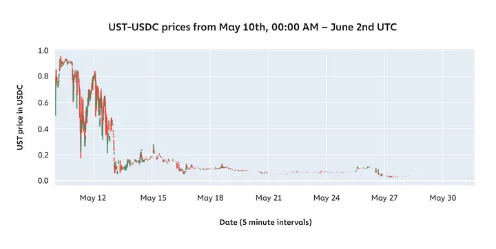
Kevin Zhou foresaw the inefficiencies within Terra’s system and actually shorted (made money if the UST went below $1) the token before anyone else knew what was coming. I had the opportunity to see his talk at Consensus where he explained his philosophy. In essence, he sees algorithmic stablecoins as a “financial alchemy” where developers attempt to create stable value out of essentially nothing. The death spiral of $UST can be seen in the line chart below.

To see Kevin’s thoughts on the future of DeFi post-Terra, check out this interview here.

All of this being said, stablecoins as a type of financial tool are still relatively new.. Some have a stronger pattern of behavior than others with new technologies offering high risk with high reward.

Stableswaps

Within decentralized markets, almost all trading activity is routed through decentralized exchanges. These are smart contracts that trustlessly exchange one asset in one liquidity pool for another asset in the same pool. As the ratio of assets changes, their comparative value also adjusts. This is no different from how the price of gasoline goes down as more gasoline is produced for the markets. As more of a digital asset is exchanged in one pool for the other, its value decreases as well. The pools are not one-to-one, however, as those markets would become very inefficient. To address this, the creators of Uniswap based the exchange rates of their pools on the constant product function. This equation is: k=x*y. A graph of the constant product function is shown below.

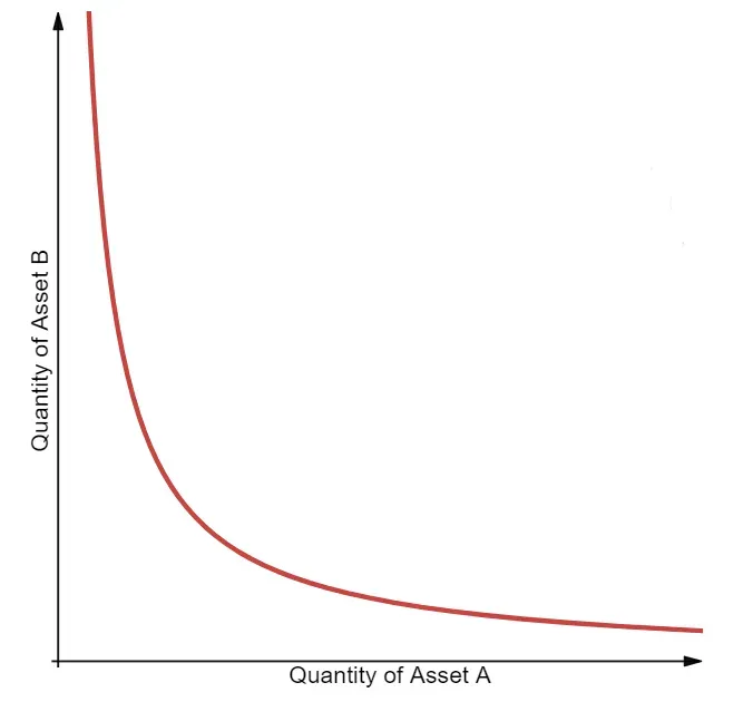
As the number of assets within the liquidity pools changes, the ratio shifts along the curve thereby adjusting the market price. As useful as this is, the constant product function is inefficient for assets that are correlated to a fixed market price, like stablecoins. Fees are higher and market prices are unnecessarily volatile for the swapping of stable assets on exchanges. Seeing this inefficiency, Michael Egorov of Curve Finance dove into the mathematics of the constant product function. His team adjusted the equation to:

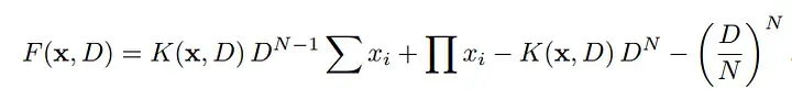
This equation blended together the constant product function with a stable curve (blue). When placed on a cartesian plane, the novel stableswap curve (orange) shows far greater price efficiency at the (1,1) price convergence ($1=$1) than does the constant product function (gray line).

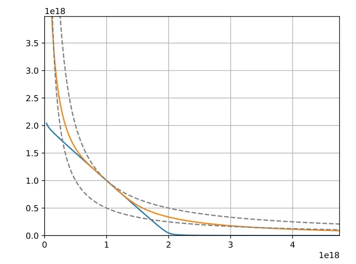
In conjunction with several other equations, Curve was able to revolutionize the way that stable assets were traded and open the market to far greater capital efficiency.

To learn more about Stableswaps on Axial and Rome Terminal, watch here.